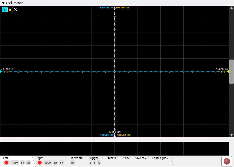
This page covers the oscilloscope's controls. For how it works inside - triggering, sin x/x reconstruction between samples, mains-hum rejection - see Theory of operation ▸ Oscilloscope.
Live time-domain view of the captured signal. Two independent
channels (L / R) share the trigger; each has its own V/div,
coupling, interpolation, and vertical offset. The capture rate
readout in the top-right corner (cap/s) shows how
many frames per second the view is rendering - or, with the
glitch trigger, how many glitches per
second have been caught (see
Capture-rate readout).
L / R
select which channel drives the
measurement table and the movable channel-offset marker - they do
not switch settings tabs. A button is disabled when
its channel is switched off in the
Left / Right
tab. L / R and Auto-Setup are always
shown; the rest appear once measurements exist
(Header buttons).0 s;
the time offset in seconds is shown above the handle. See
Trigger-offset marker.Row of square buttons at the top-left of the scope trace area. L / R and Auto-Setup are always shown; the rest (gauge, external window, stats toggle, reset) appear once measurements have been computed. There is no maximise button here.
Select which channel drives the measurement table and the channel-offset handle - they do not switch settings tabs. The button background takes the channel's trace colour when selected, and L and R are independent.
The link to the tabs runs the other way: a header button is disabled when that channel is switched off in its Left / Right tab (the per-channel enable), and re-enables when the channel is turned back on there.
One-shot fit: adjusts the time base so roughly 1.5 periods fit on screen, and the V/div so the trace spans ~75 % of the vertical area. Uses the currently-selected channel's measured period and Vpp.
Opens and closes the amplitude-histogram panel, which shows how often the signal sat at each voltage. The panel is part of this page - drag it by its title bar to move it, drag its corner to resize it - rather than a separate operating-system window, so it never disappears behind the browser and it closes when the page does. The button stays pressed while the panel is open; closing the panel releases it. Collection runs only while the panel is open.
Toggles the entire measurement table overlay on and off. When hidden, only the trace and the L / R buttons remain.
Pops the measurement table out into a separate tool window so it can sit alongside the main shell. Visible only when the table itself is visible. Closing the tool window returns the table to the main view.
Shows / hides the avg / min / max / σ columns of the
measurement table. The worker keeps computing them regardless; the
toggle only affects rendering.
Red counterclockwise-arrow button (the "roll back to the start"
reset). Clears the rolling-window statistics history that feeds the
avg / min / max / σ columns, so the next frame starts a
fresh averaging window. Useful after changing test conditions. The
amplitude histogram restarts with it -
the same events invalidate both - and so does starting or stopping the
generator.
Compact grid in the top-left of the trace area. Eight rows, up to five
value columns (cur + the four stats columns). Vmean and Vrms
are integrated over a whole number of signal periods rather than the
raw frame, so their statistics stay steady instead of wobbling with however
many part-periods happen to fit the window (see
how the numbers are
measured).
| Row | Meaning |
|---|---|
| Vpp | Peak-to-peak voltage (max − min over the visible frame). |
| Vrms | Root-mean-square voltage of the frame. |
| Vmean | DC mean - useful for spotting offsets. |
| Tp | Period (seconds), computed precisely as 1 / f from the measured frequency below. |
| Tr | Rise time (10 % -> 90 % of Vpp). |
| Tf | Fall time (90 % -> 10 %). |
| f | Frequency of the trigger-channel signal, measured to sub-sample precision; the period Tp = 1 / f is derived from it. |
| Duty | Duty cycle as % of period - high-time / period. |
Rolling-window statistics over a configurable averaging window (see Preferences -> Oscilloscope -> Measurement average). σ is the population standard deviation. The window is ~33 s at 30 fps by default; the Reset button wipes the statistics.
Every number in this table is computed on the unfiltered window - the per-channel LPF cleanup, both the 80 kHz low-pass and the de-spike median, shapes only the drawn trace. That is deliberate: those are display settings chosen to make a trace readable, and the moment one of them moves Vpp, Vmean, rise time, fall time or duty cycle, the figure stops being a measurement of the signal and becomes a measurement of our rendering of it. So you can switch the filter while watching the table and nothing in it will move. The one exception is the mains rejection, which stays in the measurement path - suppressing hum is a measurement decision, not a cosmetic one.
A capture can end without you pressing Record again - the device unplugged, taken exclusively by another application, or stopped by its driver. The scope then stops instead of drawing a flat line with the capture rate still ticking, and one Audio device error dialog names the backend and says whether the device was unplugged or its stream failed or whether it stopped delivering samples - a driver that said nothing at all, caught by the delivery deadline. The playback side is watched the same way, so a converter pulled out mid-tone stops the generator with a reason rather than leaving a lit Play button over silence. See Theory ▸ when a device won't open - and when it stops.
Opened by the amplitude-histogram button. It is a movable, resizable panel inside the page, not a window of its own. It answers a different question from the trace: not what the waveform looks like over time, but how much of its time it spends at each voltage. Voltage runs up the left axis, the number of samples counted at that level runs along the bottom, and each level is drawn as a horizontal bar.
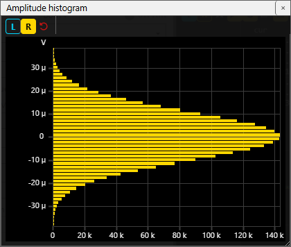
Above: a converter's own noise floor, a few tens of microvolts wide - a clean Gaussian. A bell that is visibly not Gaussian points at something other than thermal noise.
The shape is the reading:
| Shape | What it means |
|---|---|
| Two peaks at the extremes, hollow in the middle | A sine. A sinusoid moves slowest at its turning points, so it spends most of its time near ±peak - the classic bathtub. |
| A bell centred on zero | Noise. A clean noise floor is Gaussian, and a visibly non-Gaussian bell points at something other than thermal noise. |
| A tall spike at one or both ends | Clipping. Samples pinned to the rail pile into the outermost bar. |
| Unequal bars above and below the centre | Asymmetry - a one-sided clip, or an asymmetric distortion. |
The voltage axis is relative, and its middle is always 0 V. Samples are counted exactly as captured - nothing is subtracted from them and nothing is filtered - and the axis is then read from the distribution's own mean. So a DC offset on the card changes what the axis is measured from, not which level a sample is counted at, and the picture neither slides off the plot nor changes shape. Both halves are always the same height, so an asymmetric waveform shows as unequal bar lengths above and below the middle.
The resolution follows the signal, not the converter. The voltage range is sized from the signal's own peak, so a millivolt notch residual is resolved just as finely as a full-scale tone. Both axes auto-range as counts accumulate, and levels so lightly populated that they would draw as a single pixel are trimmed from the ends, so the distribution fills the window instead of being squeezed by empty tails.
The window is resizable and the plot scales with it. Its top-left corner carries:
| Control | Function |
|---|---|
| L / R | Which channel is shown - one at a time. A channel switched off in the scope is greyed and cannot be picked; if it was the one being shown, the window moves to the other. The choice is remembered between sessions. |
| Reset | Clears the collected distribution and nothing else - the measurement table's statistics are left alone. Use it to re-range onto a signal that has become much smaller, since a shrinking signal keeps the range it was given. |
Collection is unbounded while the panel is open, so a distribution can be built over minutes. It survives a V/div change, a range switch and a recalibration - recalibrating relabels the axis rather than recounting. It restarts by itself only when the level moves far enough that the old counts describe a different signal, and along with the measurement statistics when those are reset (see Reset statistics).
The count along the bottom is of samples binned, not of every sample captured: collection runs at the measurement cadence and skips blocks when the machine is busy. That is an unbiased sub-sample, so it changes how fast the bars grow but not the shape they grow into. Read the axis as relative occupancy, not as a sample census.
The number of bars is set under Preferences -> Oscilloscope -> Histogram bins (default 50). It is display resolution only: the underlying collection is far finer, so changing it re-draws what has already been collected rather than discarding it.
A horizontal marker line whose triangle handle is on the right edge. The marker can be moved only by dragging that handle up or down; double-clicking the handle returns it to the vertical centre. The current trigger level (in volts, for the active trigger channel) is shown next to the handle. Hidden while a file is loaded (a static signal has no trigger).
A vertical marker line whose triangle handle is on the bottom edge.
It sets where in the window the trigger event sits. Move it only by
dragging the handle left / right; double-click returns it to the
centre (0 s). The time offset in seconds is shown
above the handle. Hidden in file mode.
Each enabled channel has its own vertical-offset marker (dashed zero-line + triangle handle), and both handles are on the LEFT edge. The offset voltage is shown beside each handle. Only the currently-selected channel's marker is draggable - the other channel's handle is dimmed and shown for reference only. Move the active marker by dragging its handle; double-click recentres it.
A vertical scrollbar on the right pans the trace up / down (the voltage offset, both channels together). A horizontal scrollbar along the bottom pans left / right through time. Each scrollbar pans one axis only - it never zooms - but its thumb is resized by the view to show the visible fraction, so it tracks zoom: change V/div or t/div and the thumb grows or shrinks to match. Click the empty track to page toward the pointer, or hold the button down to keep paging until the thumb reaches the cursor. Zoom with the mouse wheel over the canvas.
The horizontal scrollbar appears only when an audio file is loaded - it is there to move a long recording left / right. During live capture there is nothing earlier to scroll back to, so it stays hidden.
Pale-grey figure in the top-right corner of the trace area. With the
edge trigger it shows how many new frames per second the view is
rendering - a smoothed rate that sinks toward zero while nothing
triggers. With the glitch
trigger it becomes a cumulative glitches-per-second counter:
the total number of glitches caught divided by the time spent recording,
shown to three decimals so an event every few minutes still reads e.g.
0.008 instead of rounding to zero. The count starts afresh
when the glitch type is entered or a new record starts, and the readout
stays visible for the whole record - even while reading
0.000. When recording stops, the last value stays
frozen on screen until the next record. Hidden while a file is
loaded (nothing is being captured).
The settings-tab strip at the bottom of the pane holds per-channel, trigger and utility settings. The Left, Right, Horizontal and Trigger tabs paint a row of tiles under the tab label showing their key values while the tab body is collapsed; the Presets / Utility / Save / Load tabs carry no tiles.

Controls for the left channel. Contains the channel toggle, V/div selector, AC/DC button, Sin/Lin checkbox, Residual checkbox, and the per-channel Mains and LPF drop-downs. Same layout for the Right tab.
Square toggle that enables / disables the channel. When off, the trace isn't drawn and the channel can't be picked as the trigger source.
Vertical resolution, as a 1-2-5-10 list from 1 µV/div to
500 V/div. The wheel / arrows / ↑↓ keys step through the list;
you can also type any value (with a µV / mV
/ V suffix) for a setting off the list. Independent per
channel.
AC mode subtracts the running DC mean from the displayed trace so a small AC component on top of a large DC offset is visible. The underlying measurements are still computed on the raw samples - only the displayed trace is shifted.
Per-channel checkbox shown with a small sinc-shape image. When checked, the trace is rendered with Lanczos sinc interpolation (proper bandlimited reconstruction); when unchecked, straight-line interpolation between samples. It only makes a visible difference when adjacent sample points are at least ~2 px apart on screen (i.e. zoomed in on the time axis); closer than that, the two look identical and sinc just costs more CPU.
Per-channel checkbox. When checked, the channel's trace is replaced by the residual: the captured signal minus a best-fit single tone. The tone's frequency comes from the scope's frequency measurement, and its amplitude and phase are fitted over the displayed window - so the synthesized tone is phase-aligned with the triggered display, and what remains on screen is the distortion, noise, hum and glitches that hide under the fundamental. The DC level is preserved - only the tone is taken out - so use AC if you want the residual centred on zero.
The residual works with a dual-tone signal too. The two frequencies are measured from the captured signal itself (seeded from the generator's values, then refined on the capture) - which makes the subtraction immune to the DAC and the ADC running on different clocks; the generator's values are used only until a measurement is available. The seed is what the generator says it is emitting, not what you typed into its fields, so a bin-snapped tone, a rectangle or triangle rendered at the nearest whole-sample period, and a tone running on a bench across the network all start the fit from the frequency actually going out; the same answer feeds the reconstructed-beat overlay. Both tones are fitted - the two fits refined alternately so neither leaks into the other - and both are subtracted, leaving the intermodulation products, noise and glitches under the tone pair on screen. The fit window is automatically sized to span at least two beat cycles of |F1 − F2|; if both frequencies are equal (no beat), the captured trace is shown unchanged.
Triggering and the frequency / period readouts still work on the captured signal, and the Vpp / Vrms readouts also still describe the captured signal - only the trace changes. With Auto-Setup, a channel showing its residual takes its vertical scale from the residual's peak-to-peak value, while the time base and trigger are still derived from the captured signal. When the settings-tab strip is collapsed, the channel's tile shows a residual marker while the mode is on.
A channel in residual mode gets no reconstructed-beat overlay - the beat envelope belongs to the very tones the residual has just taken out.
Drop-down that applies a per-channel mains-hum rejection filter, tracked live at the line frequency (50 / 60 Hz and its harmonics). It filters what the trace shows and what the trigger and the measurements act on, while the DC level is preserved. Four options:
How the tracked comb works is covered in the Theory of operation.
Drop-down that applies a per-channel high-frequency cleanup to the displayed trace. Three options:

Identical layout to the Left tab - channel toggle, V/div, AC/DC, Sin/Lin and Residual, but for the right channel.

Horizontal resolution, as a 1-2-5-10 list from 1 µs/div to
1 s/div (no ns/div). The wheel / arrows / ↑↓ keys step the list,
or type any value (µs / ms / s)
for a setting off the list. The trace centre stays put on a t/div change
- only the visible window's width changes.

Pair of L / R toggles picking which channel drives the trigger comparator.
↑ / ↓ pair. Rising edge triggers when the signal crosses the trigger level going up; falling edge for going down. With the glitch type the same pair picks the display anchor instead: ↑ anchors the display on the start of the glitch (the last clean sample before the break), ↓ on its end (the first settled sample after it).
E / G pair choosing what the trigger reacts to.
The glitch detector does not use the trigger level - it predicts each
sample from the sinusoid's own recurrence and fires when the prediction
error stands well clear of the noise floor, so it catches faults far too
small to reach any edge level. The level marker and
hysteresis therefore play no part
in glitch mode. Break points closer together than 1 ms merge into
one event, so a dropout's entry and recovery count as a single glitch.
While the glitch type is active, the cap/s readout turns
into a cumulative glitches-per-second counter (see
Capture-rate readout). For how the detector
tells a genuine break from noise, see
Theory of operation ▸
Oscilloscope ▸ Triggering.
A / N / S - Auto, Normal, Single.
The glitch type works only in Normal and Single - in Auto the display free-runs and would overwrite a caught glitch immediately, so switching to Auto forces the type back to edge and greys the G button out.
Active only when the mode is Single. Pressing it arms the next single-shot capture.
Checkbox + step selector in division units (0.0 .. 5.0 in 0.1
steps). Schmitt-style trigger hysteresis: a rising-edge
trigger fires only when the signal first dropped below
(level − hyst) and then crossed above
(level + hyst). This stabilises the trigger on a weak or
noisy signal - without it, noise around the level causes a flurry of
false triggers and a jittery trace. The selector greys out when the
checkbox is off; the value is preserved when toggled. Applies to the
edge type only - the glitch trigger
ignores level and hysteresis alike.
Checkbox, enabled only when the generator is in Dual tone form (greyed out for every other waveform). When on, the scope overlays the dimmed |f₁−f₂| beat envelope of the two tones on top of the live trace, so you can see the slow beat the two close tones produce and stabilise the trigger on it. The overlay is drawn per shown channel, each in a dimmed shade of that channel's own trace colour, so every dual-tone trace carries its own visually paired envelope.
It is hidden in two cases: while the generator is stopped (with no tones playing there is no beat, and the reconstruction would only trace noise), and on any channel that is showing its residual (the envelope belongs to the tones that channel has just removed).

Save and recall complete scope set-ups. In the name field type a name for the current configuration and press Save - it stores every per-channel and per-trigger setting (V/div, AC/DC, Sin/Lin, t/div, trigger channel / edge / mode, hysteresis enable + value). To restore one, pick a previously-saved name with the arrow on the right of the field and press Load. Delete removes the selected preset (after a confirmation).

Renders the scope pane to a PNG at a chosen resolution and lets you save it to disk (or copy it). The render uses an offscreen replica of the pane with the settings tabs collapsed (so the trace dominates), and at the chosen size - independent of the visible window.
Opens the shared ADC calibration dialog, which derives the ADC's full-scale voltage from a known reference signal (a calibrator or a precision generator) and writes it into the bound card's active range. Disabled until a capture is running.
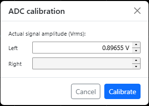
Enter the actual signal amplitude now present at the input, in
nV / µV / mV / V, and the app
scales the digital reading so that level reads true. The dialog has a
Left and a Right row for a stereo card - calibration is always
per channel, because real converter channels never match to the last
part-per-million - and a single row for a Mono card. Only the row for the
currently measured channel is live; the other channel's row is shown
disabled and empty (the shot above is a right-channel-only capture).
Calibrate the other channel by measuring it in turn - each row writes only its
own channel's active range. A card set
to Coupling: Linked is
calibrated per channel just the same - Linked couples only which range is
selected, never the measured values.

Writes the most recent capture to an audio file. The duration field (a single input in seconds) sets how much to save; the open-file button picks the destination; the Save button writes the file.

Plays back an audio file as the scope's data source instead of the live
ADC. The open-audio button picks the file - any
WAV / AIFF / FLAC, not only files
this scope saved. This is a plain waveform viewer for the file:
no triggering or measurements are available on a loaded signal, and
the FFT analyser does not run over the scope-loaded audio. The
whole file is decoded into memory (16 bytes per sample frame); a file
that cannot fit the Java heap is refused up-front, with the required and
free amounts shown.
The Left, Right, Horizontal and Trigger tabs show a row of small tiles under the tab label with that tab's key values (the other tabs have none). Tiles are passive and have tooltips explaining the value they show; they stay visible even when the tab body is collapsed.
An LED tile on the Left / Right tab, shown only while that channel is enabled (absent when the channel is off).
The channel's vertical resolution, short form (e.g. 1m,
500m, 1).
ac or dc - the channel's coupling.
sin when sinc interpolation is on, lin
when off.
The horizontal resolution, short form - e.g. 200u,
1m, 20m.
L or R - which channel is currently used to arm
the trigger.
↑ for rising, ↓ for falling. With the glitch type: anchor on the glitch's start (↑) or end (↓).
G - shown only while the
glitch trigger is selected. The absence
of this tile means the edge type.
A, N or S - Auto, Normal, Single.
Shown only when hysteresis is enabled; the number is the hysteresis window
in divisions (e.g. H 2.0). The absence of this tile means
hysteresis is off.
The trace can be moved and scaled on both axes. Everything below works the same way whether the scope is live (recording), stopped (showing the last captured buffer) or showing a loaded file - the only difference is that a live capture keeps adding new samples while the other two are frozen. The two axes are fully independent: a horizontal action never moves or rescales the trace vertically, and a vertical action never touches the horizontal.
The plain wheel, or dragging an offset handle on either side edge, moves both active channels together, keeping their spacing. You can move the signal until ±FS/2 - the converter's full-scale edge - reaches the middle of the screen; that is far enough to park any part of the signal at centre, and no further.
500 µV/div, right 1 mV/div: one
zoom-in steps the right to 500 µV/div and scales the left to
250 µV/div (50 µV off the 200 µV rung), rather than
stepping the left to 200 µV/div and scaling the right to
400 µV/div (100 µV off 500 µV). A manually-set,
off-sequence channel likewise scales in proportion to the channel that steps.Drag with the left button across the trace to draw a rectangle; release, and the selection stretches to fill the whole view - the one gesture that rescales both axes at once. A selection smaller than 8 pixels either way is ignored, so a stray click does nothing. The drag must start on the open plot area - not on a marker handle, a header button or an axis label. It works the same whether the scope is live, stopped or showing a loaded file, and the same gesture zooms the FFT and frequency-response views too (the condensed strip in a split layout is not zoomable).
With Preferences ▸
Oscilloscope ▸ Display persistence set to anything but
Off, every swept trace lingers and fades like the phosphor
of an analog scope, so trigger jitter and noise pile up into a visible
envelope. Decay times of 0.5, 1, 2, 5, 10, 15 and 20 s are offered,
plus ∞ (traces never fade) and a manual value. Persistence is
drawn on the GPU and needs WebGL2 with the
EXT_color_buffer_float extension; where the browser or the
graphics driver does not offer that combination it silently falls back to a
non-persisting trace - the setting stays available and simply has no
visible effect.
The afterglow follows a few rules so it never shows stale geometry: